NoSQL database

RDBMS features: ACID
A: Atomicity
C: Consistency
I: Isolation
D: Durability

NoSQL is used to store super large scale data. These data doesn’t need a fix pattern, just scale out.

Distributed system CAP theorem: it cann’t be satisfied three of them at the same time.
Consistency: all nodes has same data at the same time
Availability: guarantee response no matter success or fail
Partition tolerance: system keep operating even part information lost.

Categories
Column-based:
-HBase, Cassandra;
-Easy to compress data; fast-search for a certain column.

Document-based:
-MongoDB, CouchDB
-Storage Format is similar to JSON(K/V Pair), Content is document format.

Key-Value:
-Redis, Memcache
-Search value through key no matter the type of value

Column-oriented

Traditional relational database is row-oriented. Each row has a row id and every field store in one table.

When searching in row-oriented database, each row will be traversed, no matter a certain column data is needed or not. If you search a person whose birth month is September. Search row by row to target data.

Index the target column can promote search speed, but index each column cause extra overload and databse will traverse all columns to search data.

Column-oriented database will stores each column seperately. It’s very fast to search when the data amount is small. Search column by column to targetdata.

This design looks like adding index for each row. It sacrifices space and writing more index to speed up searching ability. Index maps row ID to data, but column-based database maps data to rowID. Like the picture above, it is easy to search who like archery. This is an inverted index.

When to use row-oriented and when to use column-oriented? Column-based database is easy to add one new column, but is difficult to add one row. Therefore, row-oriented database is bettern than column-based on transaction. Because it achieves real-time update. It is commonly used in marketing business.

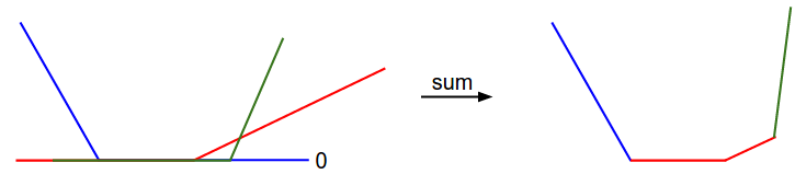
Column-oriented database has advantage of data analysis, like sum of values. Batch processing can adopt column-oriented database at night, and it supports quick search and MapReduce aggregation.

Compared to RDBMS
If you want to get all infomation of one user, column-based database costs more;
If you want to get one piece of information of one user, row-based database costs more.

Row-based is faster than Column-based on Updating a target row;
Column-based is faster than Row-based on Searching part of information of users;

Row-based database: OLTP
Column-based database: OLAP

K/V stores

This is the easiest store in NoSQL databases.

the complex k/v paire is like:

Document-oriented stores

Store based on K/V pair, but structure more complex.

MongoDB

Written in C++
Remains some friendly properties of SQL.(Query, index)
Support secondary index
Master-slave replication
Queries support javascript expressions
Better update-in-place than CouchDB
Sharding built-in
Uses memory mapped files for data storage
After crash, it needs to repair tables
Reads faster than wirtes

Use: need dynamic search. Dedine indexes first, no need map/reduce.

Example: Adapts all situations of MySQL and PostgreSQL

Cassandra

Written in Java
Querying by column
Writes are much faster than reads
Column-based databse.
Weak consistency; High availability; High scalability

Use: adapts to implement in write action more than read action

Example: Logging system, Banking system, Finance system.

HBase

Written in Java
Billion row level and Million column level
Map/Reduce with Hadoop
Store in HDFS
No single point of failure
Strong consistency; Low availability; High scalability

Use: Big table, random and real-time read/write action

Example: Facebook message database

Redis

Written in c/c++
Blazing fast
Disk-backed in-memory database
Master-slave replication
Store as key/value format
Support set, list, hash
Has transactions
Value can be set to expire
Publish/Subscribe and Watch

Use: if data is not huge and changes frequently, store in Redis. Fast read/write data

Example: Stock price analysis, Real-time data processing

Message Queue

Message Queue is a type of technique to exchange information in distributed system. MQ can stay in memory or disk until it is being read. In distributed computing system, to achieve effective information exchange, developer needs to build a communication way for asychronous network.

Communication approaches

1. Point to point: one2one, one2many, many2many
   One message only can be used once, then remove from the queue.
2. Multiple to multiple
   One message can be used multiple times.
3. Publish/Subscribe：
4. Cluster

Kafka

Kafka is a fast, scalable, persistent and highly fault-tolerant distributed publish-subscribe messaging system. Kafka supports high volumn of data and high response in demand better than JMS, RabbitMQ and AMQP. Compared with them, Kafka has higher throughput, more stable and better replication.

It can be used to obtain, analyze and stream processing with Flume, Spark Streaming, Storm, HBase and Flink together. It provides streaming data for Hadoop Big Data Lake. Kafka has low latency in Hadoop and Spark.

Advantages of Kafka

1. Reliability
2. Scalability
3. High performance

Terms

Broker: Server. Kafka cluster contains one or more servers.
Topic: Each message that sends to Kafka cluster has a category, which is called Topic.
Partition: Physical conception; Each topic has one or more partition.
Two strategies: 1. Key Hash algorithm; 2. Round Robin algorithm
Producer: Response to send message to Kafka broker
Consumer: Response to retrieve message from Kafka broker
Consumer Group
Zookeeper: Kafka relies on Zookeeper cluster save metadata for load balancing.
Offset: Index

Architecture

Producers send messages to Brokers;
Leader Broker gets and writes message into target topic to achieve persistency, and sets expire time.
Leader Broker delivers Follow Broker as replication;
Consumers retrieve messages from Brokers

Compare to Flume

1.
Flume is designed to send message to HDFS and HBase.
Kafka is a general-purpose system.
2.
Flume has many sources and sinks, but Kafka doesn’t.
If data source has been determined, just use Flume; Otherwise, adopt Kafka.

3. Flume can process data in real-time by intercepter(Filter data)
   Kafka needs an external system to help processing.
4. If data node failed, Flume cannot visit this node until node has been fixed, but it doesn’t happen in Kafka. Because Flume doesn’t have replicalition.

Implements

1. Message Queue: enough to rival traditional message system like ActiveMR and RabbitMQ
2. Behaviors tracking: Track users’ behaviors from browsing websites and searching. Saving into topic by Publish/Subscribe mode.
3. Metadata monitoring: Data monitoring
4. Log collecting: Other products like Scribe, Apache Flume.
5. Streaming processing: Products like Storm, Samza
6. Event source:

Reference

Kafka principles
Kafka Introduce
kafka详解
Kafka概念

SQL JOIN

Join clause is used to combine records from two or more tables in database.

Optimization:

on is better than where. on clause (A left join B on …) determines how to retrieve rows from table B. where will be used after this period. So try to use where less and satisfy condition on.
Pass:

1
2
3
4
5
6
7
8
9
10
11
12

mysql> SELECT * FROM product LEFT JOIN product_details
       ON (product.id = product_details.id)
       AND product_details.id=2;
+----+--------+------+--------+-------+
| id | amount | id   | weight | exist |
+----+--------+------+--------+-------+
|  1 |    100 | NULL |   NULL |  NULL |
|  2 |    200 |    2 |     22 |     0 |
|  3 |    300 | NULL |   NULL |  NULL |
|  4 |    400 | NULL |   NULL |  NULL |
+----+--------+------+--------+-------+
4 rows in set (0.00 sec)

Great:

1
2
3
4
5
6
7
8
9

mysql> SELECT * FROM product LEFT JOIN product_details
       ON (product.id = product_details.id)
       WHERE product_details.id=2;
+----+--------+----+--------+-------+
| id | amount | id | weight | exist |
+----+--------+----+--------+-------+
|  2 |    200 |  2 |     22 |     0 |
+----+--------+----+--------+-------+
1 row in set (0.01 sec)

Pass:

1

insert into t1(a1) select b1 from t2 where not exists(select 1 from t1 where t1.id = t2.r_id);

Great:

1
2
3
4

insert into t1(a1)  
select b1 from t2  
left join (select distinct t1.id from t1 ) t1 on t1.id = t2.r_id   
where t1.id is null;

Reference:

https://blog.csdn.net/u012861978/article/details/52203818

Common used architectures

AlexNet:

VGG16:

VGG19:

GoogleNet:

Inception:

Performance of CNN models:

The deeper model performs worse, but it’s not caused by overfitting.

Hypothsis: the problem is an optimization problem, deeper models are harder to optimize.

Solution: ResNet.

ResNet:

Residual block:

Complexity

The best in the left: Inception-v4: ResNet+Inception
For the right:

• VGG:Highest memory, most operations
• GoogleNet: Most efficient
• AlexNet: Smaller compute, still momory heavy, lower accuracy
• ResNet: Moderate efficiency depending on model, highest accuracy

Forward pass time and power consumption

Reference

http://cs231n.stanford.edu/slides/2018/cs231n_2018_lecture09.pdf

When NNs don’t work, we have many choices:

1. Fetch more data
2. Add more layers to NN
3. Try some new approaches in NN
4. Train longer(increase the number of iterations)
5. Change batch size
6. Try regularization
7. Chcek Bias Variance trade-off to avoid under and overfitting
8. Use more GPUs for faster computation

Architecture:
classification: VGG, ResNet, DenseNet…
segmentation: FCN, Dilated Convolution, Mask RCNN
detection: Faster-RCNN, YOLO, SSD…
image generation: UNet, Dilated Convolution, DCGAN, WGAN

Loss curve:

Regularization:
Dropout, weight decay

l1 distance is Manhattan Distance.
l2 distance is Euclidean Distance.

l1 norm(is also called Lasso Regression) is
l2 norm(is also called Ridge Regression) is

Activation function: squashes number to a range. Smooth to find best gradient direction.

Batch normalization: do it before activation function. zero-centered and range from [0.1] commonly.

to prevent gradient vanish;
to promote learning rate
to reduce dependency from initialization.

Regularization:

1. Add term to loss
   L1 Regularization;
   L2 Regularization;
   Elastic net(L1+L2)

2. Dropout

Score function -> Loss function -> Optimization.

Recall that SVM was formulated as:

This formula archieves a very low loss L. Optimization is the process of finding the set of parameters W that minimize the loss function.

Visualizing the loss function

For high-dimensional spaces, linear classifier weight matrix is difficult to visualize. However, we can gain some intuitions about one by slicing through the high-dimensinal space along rays(1-dimension) or along planes(2-dimensions).

Left: one-dimensional loss by only varying a. Middle and Right: two-dimensional loss slice, Blue = low loss, Red = high loss. The loss is piecewise-linear structure.

For single example, we have:

We can visualize this as follows:

x-axis is a single weight and y-asix is the loss.

Th picture above has shown an example of a convex function.

Optimization

The goal of optimization is to find W that minimizes the loss function.

Strategy 1: Random search(very bad)

Try out many different random weights and keep track of what works best.

Strategy 2: Random local search

Start out with a random W, generate random perturbations &W to it and if the loss is lower.

This strategy is better, but still wasteful and computationally expensive.

Strategy 3: Following the Gradient

Find a direction in the weight-space that would improve our weight vector. I means we can compute teh best direction along which we should change our weight vector that is mathematically guaranteed to be the direction of the steepest descend.

In one-dimensional functions, the mathematically expression is:

Gradient check: unlike the numerical gradient it can be more error prone to implement, which is why in practice it is very common to compute the analytic gradient and compare it to the numerical gradient to check the correctness of your implementation.

SVM loss function for a single datapoint:

We can differentiate the function with respect to the weights.

Gradient descent

Mini-batch gradient descent: batch training
Stochastic gradient descent(or on-line gradient descent): mini-batch contains only a single example.

Reference

http://cs231n.github.io/optimization-1/

Keywords: Socre function, Loss function, Bias trick, SVM classifier, Softmax classifier

Image classification of parametric approach has two major components:

1. Score function: maps the raw data to class scores.
2. Loss function: quantifies the agreement between predicted scores and the ground truth labels.

Optimization: minimize the loss function with respect to the parameters of the score function.

Linear Classifier definition:

Score function:

In the above equation, we assume that images Xi has shape [D1], W has shape [KD] and vector b (of size [K1]). In CIFAR-10, Xi has shape [30711], W has shape [103072], and b is [101], so 3072 numbers input into the function and 10 numbers come out.

Notes:

1. computed scores match the ground truth labels acros the whole training set. Intuitively, we wish that the correct class has a score that is higher than the scores of incorrect classes.
2. this approach is that the training data is used to learn the parameters w and b, but once the learning is complete we can discard the entire training set and only keep the learned parameters. Because a new test image can be simply forward through the function and classified based on the computed scores.
3. Classifying a test images involves a single matrix multiplication and addition, which is significantly faster than comparing a test image to all training images.
4. Single matrix multiplication Wx is effectively evaluating 10 separate clsssifiers in parallel.

Interpreting a linear classifier

A linear classifier computes the score of a class as a weighted sum of all of its pixel values across all 3 of its color channels. Let’s imagine that the “ship” class might be more likely if there is a lot of blue on the sides of an image. So we expect the “ship” classifier would have a lot of positive weights across its blue channel weights, and negative weights in the red/green channels.

In this image, the scores for each class are not good at all. This set of weights seems vonvinced that it’s looking at a dog.

Analogy of images as high-dimensional points:

In high-dimensional column vectors, we can interpret each image as a single point in this space. Analogously, the entire dataset is a (labeled)set of points.

The geometric interpretation of these numbers is that as we change one of the rows of W, the corresponding line in the pixel space will rotate in different directions.

Interpretation of linear classifiers as template matching:

Another interpretation for the weights W is that each row of W corresponds to a template for one of the classes. The score of each class for an image is obtained by comparing each template with the image using an inner prodict(dot product) one by one to find the best fit.

Additionally, the horse template seems to contain a two-headed horse, which is due to both left and right facing horses in the dataset. The linear classifier merges two modes of horses into a single template.

Similarly, the car classifier seems to have merged serveral modes into a single template. In particular, the template ended up with red, which hints that there are more red cars in CIFAR-10 dataset than of any other color. The linear classifier is too weak to properly account for different-colored cars,but neural networks will allow us to perform this task.

Bias trick:

We defined the score function as:

but now we simplify it as

With CIFAR-10 example, X as shape of [30731] instead of [30721], W has shape of [10*3073].The illustration shows:

If we preprocess data by appending ones to all vectors, we only have to learn a single matrix of weights insteads of two matrices that hold weights and biases.

Image data preprocessing:

Pixel values which range from [0:255] is very common to perform normalization of our input features. In particular, it’s important to center data by subtracting the mean from every feature. In the case of images, computing a mean image and subtracing it from every image to get images where the pixels range from approximately [-127, 127]. Further common preprocessing is to scale each input feature so that its values range from [-1,1]. The zero is arguably more important.

Loss function:

Loss function is going to measure our unhappiness with outcomes. Loss function also refered to as the cost function.

Multiclass Support Vector Machine Loss:

It is a commonly used loss. SVM wants to have a score higher than the incorrect classes by some fixed margin.

We first come out the class score and abbreviate to s. The score as:

The Multiclass SVM loss for i-th example is:

If the scores s = [13, -7, 11], and the first class is the true class. Assume the hyperparameter delta is 10. The expression above sums over all incorrect classes:

First gives 0 since [-7-13+10] gives a negative number. The loss outcome is 8. In summary, the SVM loss function wants the score of the correct class to be larger than the incorrect class scores by at least by delta.

In particular, we are working with linear score functions, so we can rewrite loss function:

Wj is the j-th row of W reshaped as a column.

Hinge loss: is max(0,-) function:

Sometimes people instead using squared hinge loss SVM(L2-SVM).

Regularization:

We can do by extending the loss function with a regularization penalty R(W). The most common regularization penalty is the L2 norm:

The complete Multiclass SVM loss, which is made up of two components: data loss and regularization loss:

or

N is the number of training examples. Lambda is a hyperparameter.

The most appealing property is tht penalizing large weights tends to imporve generalization, because it means that no input dimension can have a very large influence on the scores all by itself.

The regularization only works for weights but not for biases.

Softmax classifier:

SVM is one of two commonly seen classifiers. The other one is Softmax classifier.

fi means vector of class scores. Function in parentness is softmax function: it takes a vector of arbirary real-valued scores and squashes it to a vector of values between 0 to 1 that sum to one.

Information theory:

The cross-entropy between a “true” distribution p and an estimated distribution q is defined above.

Softmax classifier is minimizing the cross-entropy between teh estimated class probabilities and the “true” distribution. Additionally, cross-entropy can be written in terms of entropy and Kullback-Leibler divergence as:

Probabilistic interpretation:

The expression as we see:

can be interpreted as the probability assigned to the correct label yi given the image xi and W. In probabilistic interpretation, we are minimizing the negative log likehood of the correct class, which can be interpreted as performing MLE(Maximum Likehood Estimation).

Practical issues:

exponentials might be very large, which can be numerically unstable. Normalization is a useful trick. The expression as we see that:

In common choice, C is to set LogC = -maxj(fj). In code:

1
2
3
4
5
6
7

import numpy as np

f = np.array([123,456,789])
p = np.exp(f)/np.sum(np.exp(f))  # overflow

f -= np.max(f)
p = np.exp(f)/np.sum(np.exp(f)) # safe to do

To be precies, SVM classifier uses the hinge loss(max-margin loss). Softmax classifier uses cross-entropy loss, which is used to squash the raw class scores into normalized positive values that sum to one. In particular, note that it doesn’t make sense to talk about “softmax loss”, since softmax is a squashing function.

SVM vs. Softmax:

A picture might help clarify the distinction:

Softmax classifier provides “probabilities” for each class:

Unlike SVM which computes uncalibrated and not easy to interpret scores for all classes, Softmax classifier allows us to compute “probabilities” for all labels. For example:
Unnormalized log-probabilities for three classes come out to be [1,-2,0]. The softmax function would compute:

Now if the regularization strength lambda was higher, W would be penalized more and this would lead to smaller weights. Suppose that weights became [0.5,-1,0]. The softmax would compute:

Practice:

The performance difference between SVM and Softmax are usually very small. Compared to Softmax classifier, SVM is a more local objective. Consider an example that archieves the scores [10,-2,3] and the first class is correct. An SVM (delta=1) will see that the correct class has a score higher than the margin compared to other classes and compute loss of zero. If they were insted [10,-100,-100] or [10,9,9] the SVM would be indifferent since the margin of 1 is satisfied and the loss is zero. The SVM doesn’t care about the details of the individual scores.

In other words, Softmax is nevery fully happy with the scores it produces: the correct class could always have a higher probability and incorrect classes always a lower probability and the loss would always get better. However, the SVM is happy once the margins are satified.

Reference:

http://cs231n.github.io/linear-classify/

Steps:

Install Node.js

Install Git

Choose the right version of operating system.
Verify if it installed successfully.

1
2

$ node -v
$ git version

If there is no right to install it, add sudo at the top.

Install Hexo

1
2

npm install hexo-cli -g
npm install hexo-deployer-git --save

First line for Hexo installation, second line for Git page deployer.

Then,type hexo init command to initialize Hexo.

Execute commands below and then access to localhost:4000 to view the effect.

1
2

hexo g
hexo s

Deploy on Github Pages

Register Github account.
Build a new repository.
Create a SSH keypair. Type $ cd~/. ssh, if shows nothing, we need to create a new keypair.
Type

1

$ssh-keygen -t rsa -C "type personal email here"

Then, just press ‘enter’ button unless you need a password.
execute clip < ~/.ssh/id_rsa.pub and paste it into Github account.


Then, add new SSH key.

Verify: $ ssh -T git@guthub.com
if it shows below, you set up well.

Then set a personal info. It doesn’t require same with Github nickname.

1
2

$git config --global user.name "type your name here"
$git config --global user.eamil "type your email here"

Copy repository SSH to root Hexo ‘_config.yml’ file

1
2
3
4

deploy:
    type: git
    repository: 'paste Github repository here'
    branch: master

Branch is default as master.

Execute

1

hexo g -d

After a while, you can browse the Github Page by typing “https://“. For new, your personal blog has been built.

Then next level is to change a beautiful theme and add more extension. These will be introduced later.

FAQ:

1.For Github repository, you need to set Github Pages as master branch not just set in Hexo. Click ‘setting’ in the repository, find ‘Github Pages’, Choose ‘master branch’ in ‘Source’.

2. If you cannot push file to Github, you should check if the rsa keypair has been copied into Github pages.

Reference:

https://my.oschina.net/ryaneLee/blog/638440
https://xuanwo.org/2014/08/14/hexo-usual-problem/#Deploy%E4%B9%8B%E5%90%8E%EF%BC%8C%E9%A1%B5%E9%9D%A2%E9%95%BF%E6%97%B6%E9%97%B4404

KNN is rarely to use in practice, but it allows us to understand classify problem.

Nearest Neighbor Classifier:

Nearest Neighbor Algorithm has two ways to classify, L1 Distance and L2 Distance.

L1 Distance is Manhattan Distance.

This formula represents distance between test image and training images.

I1 is test image, I2 is training image. test set has p images. Thus, distance of test image to all image is the sum of right side. The computing process like below:

L2 Distance uses square root to obtain distance between test image and training images. L2 Distance is Euclidean Distance

Here is the code to build a Nearest Neighbor.

1
2
3
4
5
6
7
8
9
10
11
12
13
14
15
16
17
18
19
20
21
22
23
24
25
26
27
28
29
30

import numpy as np


class Nearest_Neighbor(object):
    def __init__(self):
        pass

    def train(self, X, y):
      self.Xtr = X
      self.ytr = y

    def predict(self, X):
        """ X is N x D where each row is an example we wish to predict label for """
        num_test = X.shape[0]
        # lets make sure that the output type matches the input type
        Ypred = np.zeros(num_test, dtype=self.ytr.dtype)

        # loop over all test rows
        for i in range(num_test):
            # find the nearest training image to the i'th test image
            # L1 distance
            l1_distances = np.sum(np.abs(self.Xtr - X[i, :]), axis=1)  # acc: 38.6%
            # L2 distance
            l2_distances = np.sqrt(np.sum(np.square(self.Xtr - X[i, :]), axis=1))  # acc: 35.4%
            min_index = np.argmin(l1_distances)  # get the index with smallest distance
            print("min_index:", min_index)
            Ypred[i] = self.ytr[min_index]  # predict the label of the nearest example
            print(Ypred[i])

        return Ypred

K-Nearest Neighbor Classifier:
KNN is easy to understand. When K=1 the classifier shows above. When K = 5, classifier gets the top 5 closest images. Intuitively, higher value of K has a smooth effect that makes classifier resistant the outliers.

Pros and Cons of Nearest Neighbor Classifier:

KNN:

Pros:
Simple to implement and understand.

Cons:
1.Pay much computational cost at test time, but takes no time to train.
2.Remember all training set and store it for future use.
3.Images that only has difference in light intensity are very different from pixel-based L2 computation.

Deep neural networks are very expensive to train, but it is very cheap to classify a new test example one the training is finished. This mode of operation is much more desirable in practice.

Reference:

http://cs231n.github.io/classification/